Test Compression

The test data volume increases exponentially with increase in circuit size. For large circuits, the growing test data volume causes a significant increase in test cost because of much longer test time and elevated tester memory requirements to store the test data. Therefore test compression techniques are essential to reduce the test cost by reducing the Scan patterns while trying to keep the same test quality.

Test Data Volume ≈ Number of Scan Cells in all the Scan Chains × Scan Patterns

In the International Technology Roadmap for Semiconductor (ITRS) 2013, it was predicted that more than 1000x test compression would be needed by 2020. Although there exists software techniques for test compression that are implemented by Automatic Test Pattern Generation(ATPG) tools in the form of complex algorithm, still it is not enough to achieve high test compression. Therefore we go for Hardware based test compression techniques by adding additional logic to the circuit, at the cost of increased area.

Embedded Deterministic Test (EDT)

One of the most common hardware test compression technique is EDT. Tessent TestKompress is the tool that can generate the decompressor and compactor logic at the RTL level. As shown in Figure 2, the decompressor drives the scan chain inputs and the compactor connects from the scan chain outputs.

Typically when an ATPG tool generates a pattern, it target a group of faults as a result only a small number of scan flops need to take specific values. And it would use random values to fill up the unspecified scan flops that cannot improve targeted fault detection. Thus in conventional ATPG, the patterns consists of many ‘x’ or don’t care bits that increases the test data volume and loading and unloading these bits to scan chains increases the tester time.

But EDT processes the desired bits of the ATPG pattern and determines how to load them through the decompressor in the form of EDT pattern. After processing, the resulting compressed pattern (or EDT pattern) is loaded through the decompressor, and the specified bits of the ATPG pattern get loaded into its respective scan flops. A side effect of the decompressor is that all the unspecified bits get loaded with random data, this side effect is in fact the reason aiding the compression. Thus test volume decreases by not having to store these unspecified bits and many of tester cycles are saved by not having to specifically load random data.

Decompressor

The decompressor consists of a ring generator, which is basically a Ring LFSR with external inputs as shown in Figure 3. The external inputs feeding the ring generator are commonly referred as EDT channels. The outputs of the ring generator flops will connect to scan chain inputs through a phase shifter consisting of XOR gates. As discussed earlier, phase shifter helps supporting more scan chains than the degree of LFSR. Creation of the compressed pattern from the original ATPG test pattern consists of solving a set of linear equations based on the ring generator polynomial and the phase shifter connections. Inputs to the ring generator are driven from the compressed pattern stored on the ATE.

We have already discussed about the Ring LFSR and its advantages here. Now we will discuss about the advantages of external chains in LFSR. Consider a simple LFSR with external inputs as shown in Figure 4.

First ATPG is run to determine the value of S1, S2, . . , S12, then solve the linear equations (similar to How to find the seed of a LFSR discussed earlier).

Note: In the first chain (having flops S1 S5 and S9), S1 s5 and s9 values will be loaded to the chain serially such that S1 will be loaded first to the chain in the 1^st clock cycle and then will be shifted to the right in the next clock cycle and simultaneously S5 will be loaded to the chain. This continues for 3 clock cycles till all the values are loaded at its required position. And in a similar way the other 3 chains are loaded.

Refer the figure 4; in the presence of External Chains –

1st Clock cycle	2nd Clock cycle	3rd Clock cycle
S1 = Q1 ⊕ E1	S5 = Q2 ⊕ E3	S9 = S6 ⊕ E5       = Q0 ⊕ Q3 ⊕ E5
S2 = Q2	S6 = S3       = Q0 ⊕ Q3	S10 = S7         = Q0 ⊕ E2 ⊕ Q1 ⊕ E1
S3 = Q0 ⊕ Q3	S7 = S4 ⊕ S1       = Q0 ⊕ E2 ⊕ Q1 ⊕ E1	S11 = S5 ⊕ S8        = Q2 ⊕ E3 ⊕ Q1 ⊕ E1 ⊕ E4
S4 = Q0 ⊕ E2	S8 = S1 ⊕ E4       = Q1 ⊕ E1 ⊕ E4	S12 = S5 ⊕ E6         = Q2 ⊕ E3 ⊕ E6

Thus there are 12 equations and 10 variables (where variables are – LFSR seed value and external chain inputs).

Suppose the external chains are not there in the figure, then in the absence of External Chains –

1st Clock cycle	2nd Clock cycle	3rd Clock cycle
S1 = Q1	S5 = Q2	S9 = S6       = Q0 ⊕ Q3
S2 = Q2	S6 = S3       = Q0 ⊕ Q3	S10 = S7         = Q0 ⊕ Q1
S3 = Q0 ⊕ Q3	S7 = S4 ⊕ S1       = Q0 ⊕ Q1	S11 = S5 ⊕ S8        = Q2 ⊕ Q1
S4 = Q0	S8 = S1       = Q1	S12 = S5         = Q2

Thus there are 12 equations and 4 variables (where variables are – LFSR seed value).

So it is evident that the external chains introduce more variables; thus probability of solving the equations improve, implies better fault coverage as we have a better chance of solving a set of equations targeting any fault.

Compactor

Basically there are two types of Test Response compactor –

  1.  Spatial compactor [reduces the number of output pins compared to input pins]

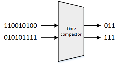
  2.  Time compactor [reduces the length of the output bit stream compared to the length of input bit stream]

EDT uses the spatial compactor which consists of group of XOR trees. It allows multiple scan chains to be observed at the same time on a given scan output channel. Several scan chains are XOR-combined into individual scan channels as shown below –

But there are two problems that we may encounter –

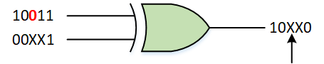
  a.  ‘X’ contamination due to unknown value propagation

Scan cells can capture unknown or’X’ values from black boxes, non-scan cells, false paths, etc. Let’s assume we have two scan chains that are compacted into one scan channel using one XOR gate, as shown below. An X captured in one of the chain will then block the corresponding cell in other chain, resulting in loss of observability.

  b.  Fault Aliasing due to bad Probability of Aliasing (PAL)

A fault is aliased when it is observed by an even number of scan cells that happened to line up at the same location in different scan chains that are compacted to the same output channel. The example shown below here illustrates this case. For this unique scenario, it is not possible to see the difference between a good and faulted circuit.

Note: Cases in which a fault is always aliased and requires a masking pattern to detect it are rare.

To deal with these issues, a mask controller is also found as a part of compactor logic. This mask controller along with masking logic at the scan chain output can selectively mask scan chains based on few bits (called mask code) at the end of the pattern shifted-in, that don’t make it to the decompressor.